CS 2770: Homework 2

Part A: Loading and Using a Pretrained Network as a Feature Extractor (30 points)

1. [2 pts] Import required modules and libraries:
   import torch
   import torch.nn as nn
   import torch.optim as optim
   from torch.optim import lr_scheduler
   import numpy as np
   import torchvision
   from torchvision import datasets, models, transforms
   import time
   import os
   import copy
   from sklearn import svm
   from sklearn.metrics import accuracy_score
   


2. [2 pts] Download the data to your home directory and preprocess the data:
   data_transforms = {
    'train': transforms.Compose([
     transforms.Resize((224,224)),
     transforms.ToTensor(),
     transforms.Normalize([0.485, 0.456, 0.406], [0.229, 0.224, 0.225])
     ]),
    'val': transforms.Compose([
     transforms.Resize((224,224)),
     transforms.ToTensor(),
     transforms.Normalize([0.485, 0.456, 0.406], [0.229, 0.224, 0.225])
     ]),
    'test': transforms.Compose([
     transforms.Resize((224,224)),
     transforms.ToTensor(),
     transforms.Normalize([0.485, 0.456, 0.406], [0.229, 0.224, 0.225])
     ]),
   }
   
   where transforms.Resize((224,224)) is for resizing all images to the same size, transforms.ToTensor() converts the input to tensor with values in the range [0,1], and transforms.Normalize([0.485, 0.456, 0.406], [0.229, 0.224, 0.225]) normalizes the tensor values based on the mean and standard deviation for RGB values. [0.485, 0.456, 0.406] contains the mean values for Red, Green and Blue channels, respectively. [0.229, 0.224, 0.225] contains the standard deviation for Red, Green and Blue channels, respectively.


3. [2 pts] Create a data loader as follows:
   data_dir = 'hw2_data'
   image_datasets = {x: datasets.ImageFolder(os.path.join(data_dir, x), data_transforms[x])
     for x in ['train', 'val', 'test']}
   dataloaders = {x: torch.utils.data.DataLoader(image_datasets[x], batch_size=8, shuffle=True, num_workers=4)
     for x in ['train', 'val' , 'test']}
   dataset_sizes = {x: len(image_datasets[x]) for x in ['train', 'val', 'test']}
   class_names = image_datasets['train'].classes
   
   where data_dir is a directory which has been created after downloading and unzipping hw2_data.zip, and contains the data for test, train and validation sets,
   image_datasets keeps the path to all images in train, val and test directories,
   dataloaders receives the image_datasets,   batch_size, shuffle and num_workers as input and returns the data loader for train, validation and test sets,
   batch_size specifies the size of mini-batch in every forward pass to the model,
   num_workers specifies how many subprocesses to use for data loading, and
   shuffle specifies whether you want to shuffle the original order of images or not.
   


4. [4 pts] Load a pretrained CNN model. The model that we are loading has been trained on 14M images from the ImageNet dataset, to classify them into 1000 classes (which aren't the same as the categories we aim to classify). To use the pretrained model as feature extractor, you need to create the following class:
   class VGG16_Feature_Extraction(torch.nn.Module):
    def __init__(self):
     super(VGG16_Feature_Extraction, self).__init__()
     VGG16_Pretrained = models.vgg16(pretrained=True)
     self.features = VGG16_Pretrained.features
     self.avgpool = VGG16_Pretrained.avgpool
     self.feature_extractor = nn.Sequential(*[VGG16_Pretrained.classifier[i] for i in range(6)])
    def forward(self, x):
     x = self.features(x)
     x = self.avgpool(x)
     x = torch.flatten(x, 1)
     x = self.feature_extractor(x)
     return x
   
   This class is of type torch.nn.Module. In the initialization, first we load the pretrained VGG16 model and then copy the features and avgpool modules. The features contains the convolutional and pooling layers. (You can find PyTorch implementation of VGG16 in this link). For our feature_extractor, we copy all the layers except the last fully connected layer from classifier of VGG16. (Note: the last fully connected layer from VGG16 is for classification on 1000 images and we do not need to have it as a part of our feature extractor). In the forward section of model, we first use the features module and then we apply avgpool. Before sending the result to the feature_extractor we need to flatten the data. Next, we use the feature_extractor to extract features.
   
   Finally, you must use the class of VGG16_Feature_Extraction(torch.nn.Module) to extract the features for all images. You need to create an instance from the VGG16_Feature_Extraction and transfer it to the cuda device:
   model = VGG16_Feature_Extraction()
   device = 'cuda:0'
   model = model.to(device)
   


5. [4 pts] Use the model to extract features of images. You can extract and save the features in different ways and here is the code of one way to do it:
   image_features = {}
   image_labels = {}
   for phase in ['train', 'test']:
    for inputs, labels in dataloaders[phase]:
     inputs = inputs.to(device)
     model_prediction = model(inputs)
     model_prediction_numpy = model_prediction.cpu().detach().numpy()
     if (phase not in image_features):
      image_features[phase] = model_prediction_numpy
      image_labels[phase] = labels.numpy()
     else:
      image_features[phase] = np.concatenate((image_features[phase], model_prediction_numpy), axis=0)
      image_labels[phase] = np.concatenate((image_labels[phase], labels.numpy()), axis=0)
   
   In this code, first we create dictionaries for image features and image labels for both test and train sets.
   Then we need to go through both train and test set, use the dataloaders which we have prepared before and extract features for every mini batch by this model_prediction = model(inputs) command. Since we want to use these features to train a SVM classifier, our features and labels must be numpy arrays. The output of model predictions are tensor on CUDA device and we need to transfer them to numpy array. The code model_prediction_numpy = model_prediction.cpu().detach().numpy() converts the tensors to NumPy arrays.
   In the last step, we save the predictions. There are two main methods for saving the images: 1) you can concatenate features and labels in every step, or 2) create a 2d array for features and labels in both test and train set. The size of array for features representation is n*4096 in which n is number of images and 4096 is size of extracted feature. (Note: The second approach is more efficient bacause it does not need concatenation in every step)


6. [8 pts] After retrieving features from the pre-trained VGG16 network, train a linear SVM using SKLearn's LinearSVC function on the train set but do not train on the withheld validation set or test set. You need to standardize the train set and test set before training and testing your SVM. You can use the sklearn.preprocessing.StandardScaler to do this.


7. [8 pts] Test your SVM on the test set (remember to standardize test features using the train mean and standard deviation first) and report the accuracy of the SVM at predicting the class (i.e. the folder that the image was in). Also include a confusion matrix of the predictions using the sklearn.metrics.confusion_matrix function and include it in your submission. Include a brief description of what you observe about the types of errors the network makes, as a text snippet in your notebook.

Part B: Train and Test the CNN on Our Dataset (30 points)

Preparing the network: [2 pts]

1. In this step instead of using the VGG16 as a feature extractor, you will train it on our dataset (PASCAL, for a classification task). To do so, first you need to load the VGG16 with pretrained weight from ImageNet.
   model = models.vgg16(pretrained=True)
   
2. Then you need to extract the number of input features for the last fully connected layer of model:
   num_ftrs = model.classifier[6].in_features
   
3. At the end, you need to replace the last fully connected layer with a new layer. This new layer has the same number of input features as the original network but the number of outputs are the same as the number of classes in our dataset:
   model.classifier[6] = nn.Linear(num_ftrs, len(class_names))
   

Steps before starting training: [2 pts]

4. Set the number of epochs to 25.
   num_epochs = 25
   
5. Send the model to CUDA device:
   model = model.to(device)
   
6. Specify the criterion for evaluating the trained model:
   criterion = nn.CrossEntropyLoss()
   
7. Set the optimizer, learning rate and momentum:
   optimizer = optim.SGD(model.parameters(), lr=0.001, momentum=0.9)
   
8. At the end, create a scheduler to control the way that learning rate changes during the training process:
   scheduler = lr_scheduler.StepLR(optimizer, step_size=7, gamma=0.1)
   

Training: [10 pts]

9. Before starting to iterate over epochs, we need to save the initial model weight as the best model weight and set the best accuracy as zero.
   best_model_wts = copy.deepcopy(model.state_dict())
   best_acc = 0.0
   
10. Now we can start to iterate over the epochs.
    for epoch in range(num_epochs):
    
11. In the next step, we need to iterate over the train and validation sets. (Note: In every epoch once you need to go through the train set for training the model parameters and then you need to go through the validation set to evaluate the trained model.)
    for phase in ['train', 'val']:
     if phase == 'train':
      model.train()
     else:
      model.eval()
    
12. In the next step we need to go through the data by using the dataloader which we have prepared in previous steps. In every iteraion, we get a minibatch of images and their corresponding labels.
for inputs, labels in dataloaders[phase]:
 inputs = inputs.to(device)
 labels = labels.to(device)

13. Before staring to use the model for predicting a mini batch, we need to initialize the gradient vector to all zeros.
    optimizer.zero_grad()
    
14. Now we need to use the current model weight for prediction and backpropagating the prediction loss.
    with torch.set_grad_enabled(phase == 'train'):
     outputs = model(inputs)
     _, preds = torch.max(outputs, 1)
     loss = criterion(outputs, labels)
     if phase == 'train':
      loss.backward()
      optimizer.step()
    all_batchs_loss += loss.item() * inputs.size(0)
    all_batchs_corrects += torch.sum(preds == labels.data)
    In the first line we use this code with torch.set_grad_enabled(phase == 'train')to enable gradient calculation in train phase.
    Then we use the model to predict the classes of every minibatch and compute the loss.
    If we are in training, we need to send the loss backward to network and update the optimizer.
    
At the end we need to sum the loss and number of correctly predicted values over all batchs.
15. After iteraring over all minibatchs and if we are in training phase, we need to run scheduler.step() to update the scheduler status as follows:
    if phase == 'train':
     scheduler.step()
    
16. In the next step we compute the loss and accuracy of the epoch.
    epoch_loss = all_batchs_loss / dataset_sizes[phase]
    epoch_acc = all_batchs_corrects.double() / dataset_sizes[phase]
    
17. At the end if we are in validation set, we check whether the accuracy of classification is better than the best accuracy so far to save the best model parameters.
    if phase == 'val' and epoch_acc > best_acc:
     best_acc = epoch_acc
     best_model_wts = copy.deepcopy(model.state_dict())
     torch.save(best_model_wts , 'best_model_weight.pth')
    

Testing: [4 pts]

18. The testing process is very similar to train process except that we do not need to backpropagate the loss. For testing the model, first we need to prepare the model in the same way that we prepared for training process and load the best model weight that we saved in training process.
    model = models.vgg16()
    num_ftrs = model.classifier[6].in_features
    model.classifier[6] = nn.Linear(num_ftrs, 20)
    model = model.to(device)
    model.load_state_dict(torch.load('best_model_weight.pth'))
    
19. After loading the model weight, we need to set the model to eval and the value of phase to 'test'.
    
model.eval()
phase = 'test'

20. In the next step, we need to go through test set, predict the category of images, and compute number of correctly classified images.
    for inputs, labels in dataloaders[phase]:
     inputs = inputs.to(device)
     labels = labels.to(device)
     outputs = model(inputs)
     _, preds = torch.max(outputs, 1)
     all_batchs_corrects += torch.sum(preds == labels.data)
    
21. At the end, we compute the accuracy over all data.
    epoch_acc = all_batchs_corrects.double() / dataset_sizes[phase]
    

Repeating with different hyperparameters: [12 pts]
22. Retrain your model with different hyperparameters / implementation details and include the confusion matrix and accuracy of the model on the test data. For example, you can play with learning rate, batch size, choice of optimizer, regularization, etc. You need to experiment with at least three different hyperparameters and two settings for each.

Part C: Object Detection (Faster RCNN) Training and Evaluation (30 points)

1. Computing the performance of object detection is more complicated compared to object classification. The output of object detection are bounding boxes and to compute the performance we use mAP (mean Average Precision). The definition of mAP is as follows:
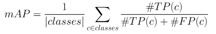         where
   
   • True Positive - TP(c): a predicted bounding box (pred_bb) was made for class c, there is a ground truth bounding box (gt_bb) of class c, and IoU(pred_bb, gt_bb) >= threshold.
   • False Positive - FP(c): a pred_bb was made for class c, and there is no gt_bb of class c. Or there is a gt_bb of class c, but IoU(pred_bb, gt_bb) < threshold.
   For a given class c, to compute the Intersection over Union metric (IoU) (see image below) between any individual predicted bounding box and the ground truth bounding boxes, take the best overlap (i.e. the highest overlap between the predicted and any ground truth box) as your final score for that predicted bounding box. If there is no ground truth bounding box, but you predict a positive window, your score for that box is 0.
   
   
   
   [10 pts] You need to write your own function to compute mAP scores, given predicted and ground-truth bounding boxes (with associated labels) as input. Needless to say, do not look up or copy solutions for this part from the web. Include your code in an appropriately named function, and use it below when needing to report mAP scores.


2. There are two datasets that you need to download, PASCAL.zip and PennFudanPed.zip, both available at the links above. For the PASCAL dataset, inside each of the train, test, and val directories, there exist three directories: 1) Images, 2) BBox and 3) Labels. The images folder contains the images from PASCAL VOC dataset, the BBox folder contains the ground truth bounding boxes of objects in every image and the Labels contains the object category for bounding boxes in every image. For PennFudanPed, there exist two directories: 1) Images and 2) Masks. The Images folder contains images from Penn-Fudan dataset and Masks folder contains the segmentation mask of objects in every image. The number of categories which are in PASCAL dataset is 5. The categories are person, bicycle, car, motorcycle, airplane and their corresponding labels are 1, 2, 3, 4, 5, respectively. In addition to these labels, label 0 belongs to category of background and as the result the total number of classes which you need to use for training process is 6.
   PennFudanPed just contains pedestrian (person) category. As the result the total number of classes for the object detection task is 2. You should also download and copy files from this zip file into your working directory: Required_Files.zip. Finally, the assignment also relies on this API.


3. You need to import required modules and libraries:
   import torch
   import torchvision
   from torchvision.models.detection.faster_rcnn import FastRCNNPredictor
   from pascal_dataset import PASCALDataset
   import utils
   from coco_utils import get_coco_api_from_dataset
   from coco_eval import CocoEvaluator
   import copy
   import torch.optim as optim
   from torch.optim import lr_scheduler
   from PennFudanDataset import PennFudanDataset
   


4. To represent our datasets, we have prepared the PASCALDataset class in pascal_dataset.py and PennFudanDataset class in PennFudanDataset.py. You can use these classes in your code as follows:
   dataset = PASCALDataset('path_to_data')
   dataset = PennFudanDataset('path_to_data')
   Note: The path to data is the path to train, test, or val sets NOT the directory which includes the whole dataset. As the result, you need to create a separate dataset for each of train, test and validation sets.
   


5. Next, create the data loader, for example by:
   data_loader = torch.utils.data.DataLoader(dataset, batch_size=4, shuffle=True, num_workers=4, collate_fn=utils.collate_fn)
   where collate_fn=utils.collate_fn. collate_fn=utils.collate_fn is used to return the tuples of images and image annotations in every iteration.
   


6. Load the pre-trained detection model:
   model = torchvision.models.detection.fasterrcnn_resnet50_fpn(pretrained=True)
   The number of classes in pre-trained model is different from the number of classes in our datasets. So similar to what you did in homework 2, you need to replace the box_predictor of model with a new FastRCNNPredictor layer to predict 6 classes when you are training on PASCAL dataset and 2 classes when you are training on PennFudanPed dataset.
   Before starting the training process you need to set the optimizer, scheduler and number of epochs as before.


7. [6 pts] Now you can start to train the network and in every epoch you have two phases of train and validation. In every epoch, if the mAP of the validation set is the largest mAP so far, you need to save the model weight. Iterate over train set to perform the training process and then iterate over the validation set to evaluate the performance of trained model. Here is the set of commands to iterate over data, prepare the images and labels, and use them as input to model for object detection task:
   for images, targets in data_loader:
    images = list(image.to(device) for image in images)
    targets = [{k: v.to(device) for k, v in t.items()} for t in targets]
    loss_dict = model(images, targets)
   First line in for loop: Since the images and targets are of type tuple, we need to convert them to a list. In the first line of for loop, first all Images in the batch are transferred to GPU device and then a list is created from all images. The input to the model is the list of all images of the batch.
   Second line in for loop: A target is a dictionary which contains the bounding box of objects, label of object, image ids, the areas of bounding boxes and whether or not the image is crowded. In the second line of for loop, all the values in dictionary of every image targets (annotations) are transferred to GPU device and finally a list is created from all targets in the batch.
   Third line in for loop: We use the the images and targets as input to the model and get the loss values. Note that the inputs to the model in train mode are both the images and the targets (annotations). Since the task of object detection has more than one loss value, the output for every image is a dictionary of all loss values. The dictionary contains following loss values: 1) loss_classifier: measures the performance of the object classification for detected bounding boxes, 2) loss_box_reg: measures the performance of network for retrieving the coordinates of the ground truth bounding boxes, 3) loss_objectness: measures the performance of network for retrieving bounding boxes which contain an object and 4) loss_rpn_box_reg: measures the performance of network for retrieving the region proposals.
   You need to sum all losses and backpropagate the loss. As before, in every iteration of training phase you need to zero the gradient and apply step function of the optimizer. After iterating over the whole train set, you need to update the scheduler.


8. [6 pts] In the validation phase you need to create a coco evaluator to evaluate the performance of the network. To create an evaluator, first you need to create a coco API from our dataset:
   coco = get_coco_api_from_dataset(data_loader.dataset)
   Then you need to specify the IoU type:
   iou_types = ["bbox"]
   At the end, you can create a coco evaluator from coco API and IoU types:
   coco_evaluator = CocoEvaluator(coco, iou_types)
   At this point, you can start to iterate over validation set and compute the mAP. In every iteration first you need to transfer the images to GPU and then use them as input to the model. The input of model in evaluation mode is just images and as opposed to train phase, you do not need to transfer the target (annotations) to GPU. Here is the command to get the object detection for the images:
   outputs = model(image)
   For evaluation in coco_evaluator, the outputs needs to be on CPU and you need to transfer them from GPU to CPU. Then you need to create the pair of target and output as follows:
   res = {target["image_id"].item(): output for target, output in zip(targets, outputs)}
   Now the res is used to update the coco evaluator in every iteration: coco_evaluator.update(res)
   After iterating over all images, you need to run the following commands to get the final results for evaluation in every epoch: coco_evaluator.synchronize_between_processes()
   coco_evaluator.accumulate()
   coco_evaluator.summarize()
   At this point you can get the mAP over all validation set by the following command: coco_evaluator.coco_eval['bbox'].stats[0]
   You need to save the model weight which has the highest mAP on the validation set.


9. [8 pts] Train networks for both PASCAL and PennFudanPed with a few different hyperparameters. Report the performance of the model which has the best test accuracy among all of your experiments (as a text snippet inside your notebook), and use it to visualize the object detection results. For your visulization, you need to write a code to draw the bounding boxes which have been detected by the network in the image. In addition to bounding boxes, the name of category and its score should be shown somewhere around the bounding box. Your code needs to find 20 images from the test set with highest mAP, draw the bounding boxes and save the outputs a directory; you will then submit these files.

Part D: Object Detection with Facebook's Detectron2 (10 points)