CS1674: Homework 7
Due: 11/1/2023, 11:59pm
This assignment is worth 50 points.
In this assignment, you will develop two variants of a scene categorization system. You will write three functions and two scripts. The first function will compute the spatial pyramid match representation. The second and third will find labels for your test images, using two classifiers: K nearest neighbors (KNN), and support vector machines (SVM). In the scripts, you will call your first function to compute the SPM representation, then compare the performance of different levels of the SPM representation, and different classifiers. Please read the entire assignment before you start working.
Download the images and SIFT features contained in the scenes_lazebnik.zip file on Canvas. This file contains the dataset split across eight folders, for eight classes/categories. All images in a subfolder (e.g. "coast") belong to the same category. For each sample, the dataset includes the image, a resized image (to be used in a later assignment) and a .mat file containing SIFT features for this image.
Next, download the load_split_dataset.m file from Canvas. This script is the first thing you should run. It assigns the following variables:
- train_images (matrix of size Mx2 where M is the total number of training images; it contains the height and width for each training image, which you need for the spatial pyramid representation),
- train_sift (a cell array of size Mx1, where each cell entry contains the values and locations of the SIFT descriptors for the training images; remember that we index cell array entries as {i} not (i)),
- train_labels (vector of size Mx1, containing the labels for each training image),
- test_images (matrix of size Nx2, where N is the total number of test images),
- test_sift (cell array of size Nx1),
- test_labels (vector of size Nx1).
There are 150 images total for each class, and this script splits them into 100 per class for training, and 50 for test. It also runs K-means to obtain a means variable (of size KxD, where K is the number of clusters and D is the feature dimensionality, explained before) which you will need. You will get a warning that K-means failed to converge-- that's ok; we can ask it to run for more iterations, but for expediency, we won't.
For each image, the corresponding .mat file contains two variables: f and d. Each column in the first variable matches a column in the second variable; both correspond to the same descriptor. You need the first two entries in each column of f to determine the (x, y) coordinates of the descriptor scored in that column of d. For reference, it's worth noting that the SIFT features for each image were extracted for you using the vl_sift function of the VLFeat package.
While the load_split_dataset script loads the SIFT descriptors, the features we will actually use to classify aggregate all SIFT descriptors per image. You will do this in computeSPMRepr, and use this representation in your compare_representations and compare_classifiers scripts, explained below. You should save your training/test features in matrices train_features and test_features of size MxD and NxD, with D defined below. You will also need the train_labels and test_labels from above.
Part I: Computing the SPM representation (10 points)
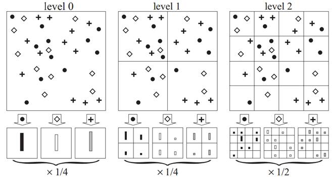
The Spatial Pyramid Match (SPM) representation was proposed in 2006 by Svetlana Lazebnik, Cordelia Schmid and Jean Ponce, and won the "test of time" award at CVPR 2016. The procedure of computing the pyramid is summarized in the following image from the paper, and described below. You will only construct the first two levels (level-0 and level-1).
Write the following: function [pyramid, level_0, level_1] = computeSPMRepr(im_size, sift, means); which computes the Spatial Pyramid Match histogram as described in class.
Inputs:
- im_size is the image size [height width] for an image,
- sift are the SIFT features for the image, and
- means are the cluster centers from the bag-of-visual-words clustering operation (computed on the training images in load_split_dataset).
Outputs:
- pyramid is a 1xD feature descriptor for the image combining the level-0 and level-1 of the spatial pyramid match representation.
- level_0 is the standard bag-of-words histogram, and
- level_1 is the bag-of-words histogram at level-1 (i.e. one histogram for each quadrant of the image).
Instructions:
- [2 pts] First, create a "bag of words" histogram representation of the features in the image, using the function function [bow] = computeBOWRepr(descriptors, means) that you wrote for HW4 (if your function does not work, you can use the one provided on Canvas). This will give you the representation shown in the left-hand side of the figure above, where the circles, diamonds and crosses denote different "words". In this toy example K = 3; in your submission, use K = 50. This forms your representation of the image, at level L = 0 of the pyramid.
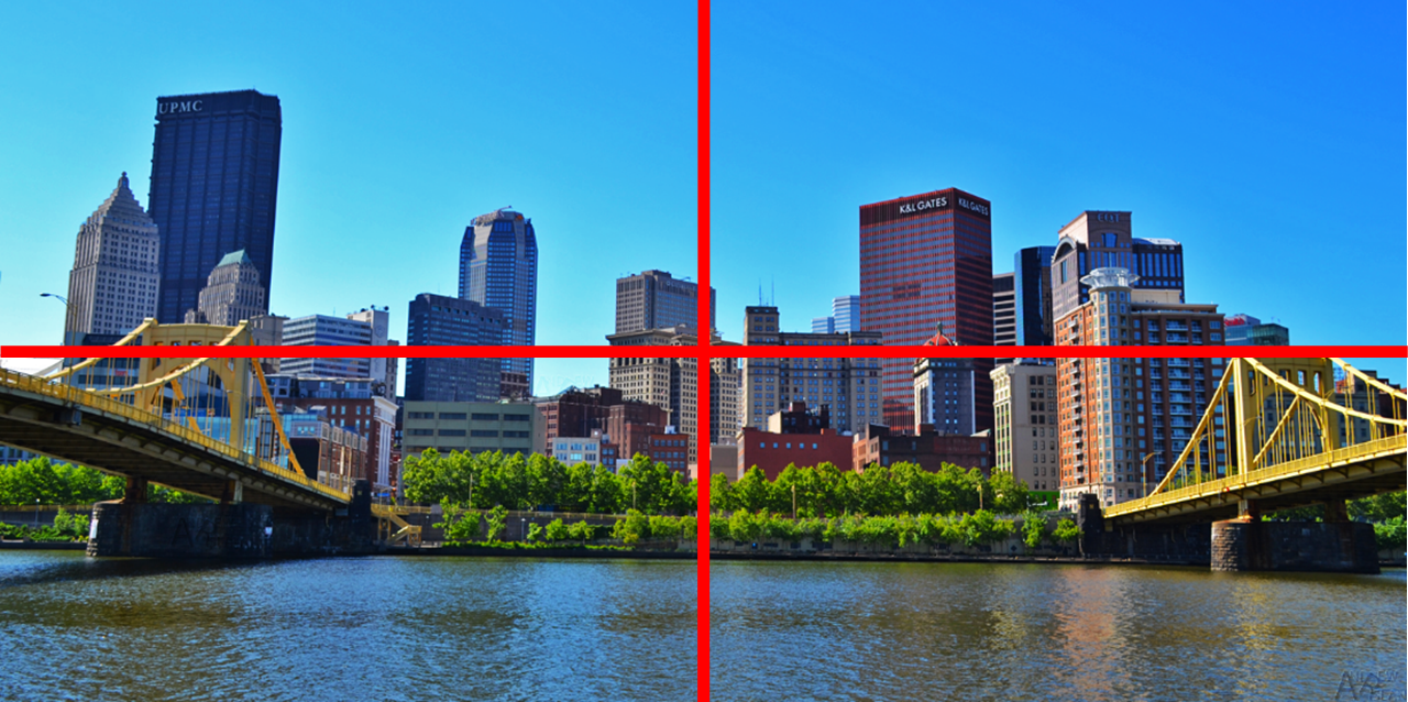
- [7 pts] Then, divide the image into four quadrants as shown below. You need to know the locations of the feature descriptors so that you know in which quadrant they fall; these are stored in the f variable in each SIFT file. Compute four BOW histograms, using the computeBOWRepr function, but generating a separate BOW representation for each quadrant. The concatenation of the four histograms is your level-1 representation of the image. The size of this representation is 1x(4*K).
- [1 pt] Finally, concatenate the level-0 and level-1 representations computed in the above steps. This will give you the final image representation, and should be saved in the pyramid variable.
Part II: Training and obtaining labels from two classifiers (15 pts)
In this part, you will write functions to obtain labels on the test data from two classifiers, support vector machines (SVM) and K nearest neighbors (KNN). (We will cycle the training or test sets as the actual test set, for comparison purposes, in Part III below.) Note that the value of k in KNN is distinct from the value K in K-means; we'll use k to denote the former and K to denote the latter.
Write the following functions:
- [10 pts] function [predicted_labels_test] =
findLabelsKNN(pyramids_train, labels_train, pyramids_test, k); which predicts the labels of
the test images using the KNN classifier. For each test image, compute the Euclidean distance between its descriptor and each training image's descriptor (the descriptors are now the Spatial Pyramids). Then find its k closest neighbors among only training images; you can use the Matlab function pdist2. Find the mode (most common value; see Matlab's function mode) among the labels, and assign the test image to this label. In other words, the neighbors are "voting" on the label of the test image. You have to write your own code, and you are NOT allowed to use the built-in Matlab function for KNN!
Inputs:
- pyramids_train, pyramids_test should be an MxD matrix
and an NxD, respectively, where M is
the size of the training image set, N is the size of your
test image set, D equals 5*K, and each pyramids(i, :)
is the 1xD Spatial Pyramid Match representation of the
corresponding training or test image.
- labels_train should be an Mx1 vector of
training labels.
Outputs:
- predicted_labels_test should be a Nx1 vector of predicted labels for the test images.
- [5 pts] function [predicted_labels_test] =
findLabelsSVM(pyramids_train, labels_train, pyramids_test); which predicts the labels of the test images using an SVM. This function should include training the SVM. The inputs and outputs are defined as above but now we will use an SVM to determine the outputs. Use the Matlab built-in SVM functions for training and test/prediction. To train a model, use model = fitcecoc(X, Y); where X (of size MxD) are your features, and Y (of size Mx1) are the labels you want to predict. To use the model you just learned, call label = predict(model, X_test); where X_test of size NxD are the descriptors for the scenes whose labels you want to predict.
Part III: Comparing approaches (25 pts)
In this part, you will compare the KNN and SVM classifiers using the SPM representation. You will also compare how the same classifier performs when it uses different levels of the SPM pyramid. Your classifiers will predict to which scene category each test image belongs.
- [10 pts] In a script compare_representations.m:
- [5 pts] Call your computeSPMRepr to compute the spatial pyramid match representation on top of the extracted SIFT features, for all train/test images. Store the resulting representations (level-0, level-1, and pyramid separately) in appropriate variables (with rows corresponding to number of samples, and columns corresponding to feature dimensions).
- [5 pts] Use an SVM classifier. Compare the quality of three representations, pyramid, level_0 and level_1. In other words, compare the full SPM representation to its constituent parts, which are the level-0 histogram and the concatenations of four histograms in level-1. Compute the accuracy at each level, by measuring what fraction of the images was assigned the correct label. In a file results1.txt, describe your findings, and give your explanation of the performance of the different representations.
- [15 pts] In a script compare_classifiers.m, do the following steps (you can interleave them as you wish, order does not have to be as shown). You can assume the previous script has been run first, so you don't have to recompute the SPM representations.
- [5 pts] Apply the SVM and KNN classifiers (i.e. call findLabelsSVM, findLabelsKNN) to predict labels on the test set, using the pyramid variable as the representation for each image. For KNN, use the following values of k=1:2:21. Each value of k gives a different KNN classifier.
- [2 pts] Compute the accuracy of each classifier on (1) the training set, and (2) the test set, by comparing its predictions with the "ground truth" labels.
- [5 pts] Plot the training and test accuracy of both types of classifiers, using the values of k on the x-axis, and accuracy on the y-axis. Since SVM does not depend on the value of k, plot its performance as a straight line. Save the result as results.png and submit it. Label your axes and show a legend. Useful functions: plot, xlabel, ylabel, legend.
- [3 pts] Finally, in a text file results2.txt, explain what you see in your plot, and explain the trends on the training and test sets you see as k increases.
Submission:
- computeSPMRepr.m
- findLabelsKNN.m
- findLabelsSVM.m
- compare_representations.m
- compare_classifiers.m
- results.png, results1.txt, results2.txt