CS1674: Homework 4
Due: 10/4/2023, 11:59pm
This assignment is worth 50 points.
Part I: Feature Description (30 points)
In this problem, you will implement a feature description pipeline, as discussed in class. While you will not exactly implement that, the SIFT paper by David Lowe is a useful resource, in addition to Section 7.1 of the Szeliski textbook.
Use the following signature: function [features] = compute_features(x, y, scores, Ix, Iy). The inputs x, y, scores, Ix, Iy are defined in HW3. The output features is an Nxd matrix, each row of which contains the d-dimensional descriptor for the n-th keypoint.
We'll simplify the histogram creation procedure a bit, compared to the original implementation presented in class. In particular, we'll compute a descriptor with dimensionality d=8 (rather than 4x4x8), which contains an 8-dimensional histogram of gradients computed from a 11x11 grid centered around each detected keypoint (i.e. -5:+5 neighborhood horizontally and vertically).
- [4 pts] If any of your detected keypoints are less than 5 pixels from the top/left or 5 pixels from the bottom/right of the image, i.e. pixels lacking 5+5 neighbors in either the horizontal or vertical direction, erase this keypoint from the x, y, scores vectors at the start of your code and do not compute a descriptor for it.
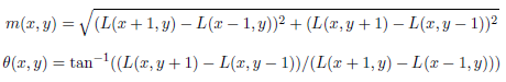
- [8 pts] To compute the gradient magnitude m(x, y) and gradient angle θ(x, y) at point (x, y), take L to be the image and use the formula below shown in class and Matlab's atand, which returns values in the range [-90, 90]. If the gradient magnitude is 0, then both the x and y gradients are 0, and you should ignore the orientation for that pixel (since it won't contribute to the histogram).
- [6 pts] Quantize the gradient orientations in 8 bins (so put values between -90 and -67.5 degrees in one bin, the -67.5 to -45 degree angles in another bin, etc.) For example, you can have a variable with the same size as the image, that says to which bin (1 through 8) the gradient at that pixel belongs.
- [6 pts] To populate the SIFT histogram, consider each of the 8 bins. To populate the first bin, sum the gradient magnitudes that are between -90 and -67.5 degrees. Repeat analogously for all bins.
- [6 pts] Finally, you should clip all values to 0.2 as discussed in class, and normalize each descriptor to be of unit length, e.g. using hist_final = hist_final / sum(hist_final); Normalize both before and after the clipping. You do not have to implement any more sophisticated detail from the Lowe paper.
Part II: Image Description with SIFT Bag-of-Words (10 points)
In this part, you will compute a bag-of-words histogram representation of an image. Conceptually, the histogram for image
Ij is a k-dimensional vector: F(Ij) = [ freq1, j freq2, j ... freqk, j ], where each entry
freqi, j counts the number of occurrences of the i-th visual word in image j, and k is
the number of total words in the vocabulary. (Acknowledgement: Notation from Kristen Grauman's assignment.)
Use the following function signature: function [bow_repr] = computeBOWRepr(features, means) where bow_repr is a normalized bag-of-words histogram (a row vector), features is the Nx8 set of descriptors computed for the image (output by the function you implemented in Part I above), and means is a kx8 set of cluster means. A set of files with cluster means are provided for you on Canvas (for k={2, 5, 10, 50}).
- [2 pt] A bag-of-words histogram has as many dimensions as the number of clusters k, so initialize the bow variable accordingly.
- [4 pts] Next, for each feature (i.e. each row in features), compute its distance to each of the cluster means, and find the closest mean. A feature is thus conceptually "mapped" to the closest cluster. You can do this efficiently using Matlab's pdist2 function (with inputs features, means).
- [4 pts] To compute the bag-of-words histogram, count how many features are mapped to each cluster.
- [2 pts] Finally, normalize the histogram by dividing each entry by the sum of the entries.
Part III: Comparison of Image Descriptors (10 points)
In this part, we will test the quality of the different representations. A good representation is one that retains some of the semantics of the image; oftentimes by "semantics" we mean object class label. In other words, a good representation should be one such that two images of the same object have similar representations, and images of different objects have different representations. We will test to what extent this is true, using our images of cardinals, leopards and pandas.
To test the quality of the representations, we will compare two averages: the average within-class distance and the average between-class distance. A representation is a vector, and "distance" is the Euclidean distance between two vectors (i.e. the representations of two images). "Within-class distances" are distances computed between the vectors for images of the same class (i.e. leopard-leopard, panda-panda). "Between-class distances" are those computed between images of different classes, e.g. leopard-panda. If you have a good image representation, should the average within-class or the average between-class distance be smaller?
A script compare_representations.m is provided for you, which does the following:
- Reads the images, and resizes them to 300x300.
- Uses the (a) code you wrote above, (b) the function extract_keypoints you wrote in HW3 (talk to the TA or instructor if that function doesn't work), and (c) another function [texture_repr_concat, texture_repr_mean] = computeTextureReprs(image, F) provided for you, to compute three types image representations (bag of words using SIFT descriptors using different values of k i.e. different number of cluster centers, concatenation of the texture representation of all pixels, and average over the texture representation of pixels) for each image.
- Computes and prints the ratio average_within_class_distance / average_between_class_distance for each representation type.
- compare_represenations calls computeTextureReprs which has the following inputs: image is the output of an imread, and F is the 49x49xnum_filters matrix of filters you used in HW2. The latter function computes two image representations based on the filter responses. The first is simply a concatenation of the filter responses for all pixels and all filters. The second contains the mean of filter reponses (averaged across all pixels) for each image.
Your task in this part is to do the following. Run compare_representations (check the top of the script for use tips); it tries different values of k. Experiment with different values for the number of keypoints you extract from images, by changing your extract_keypoints function (no need to submit any changes to it; we'll use our own function). Then, in a file answers.txt, answer the following questions.
- For which of the three representations is the within-between ratio smallest?
- Does the answer to this question depend on the value of k that you use?
- Does it depend on the number of keypoints you extract? (Try 500, 1000, 2000, 3000.)
- Which of the three types of descriptors that you used is the best one? How can you tell?
- Is this what you expected? Why or why not?
You can copy-paste ratios from the output of compare_representations as needed to support your answers.
Submission:
- compute_features.m (from Part I)
- computeBOWRepr.m (from Part II)
- answers.txt (from Part III)