CS 1501
Additional Graph and Priority Queue Notes
Prim's MST Algorithm
In lecture we discussed how Prim's MST Algorithm can be implemented effectively using the Priority First Search (PFS) code for adjacency lists shown in the text. Consider the run-time of this implementation. Recall that for each new edge (v, w) that is considered for the tree, vertex v is already in the tree and vertex w is not yet in the tree. Also recall that the priority queue (pq) is storing vertices "on the fringe" with the current "best edge" that will connect them to the tree. Thus, each time a new edge (v, w) is considered, the pq must be accessed (via the update() function). This function does the following:
· Checks to see if vertex w is in the pq.
· If w is not in the pq, add it to the pq with the priority provided (in this case equal to the weight of edge (v, w))
· If w is in the pq, and the current priority for w is lower than that provided (weight of edge (v, w)), change the priority for w to the priority provided. If the current priority for w is higher than that provided (weight of edge (v, w)), do nothing.
In calculating the run-time for this implementation, we note that (similar to DFS and BFS) we consider each edge in the graph 2 times, once from each end-vertex' point of view. This would give us a run-time of Theta(E) if consideration of an edge was a constant time operation. However, now each edge that is considered potentially causes an insert or a change in the pq, and each vertex must eventually be removed from the pq, so we can say that the total run-time is proportional to:
(E * time_to_insert_or_change_pq) + (V * time_to_remove_pq)
Based on the indirect Heap priority queue implementation discussed in Chapter 11 of the text (and, briefly, later in this handout), we know that for a pq with n items, each of the operations insert, change and remove from the pq can be done in time proportional to lg n. This causes our total time to be: Theta((E * lg V) + (V * lg V)) = Theta((E + V) lg V). Note that since E is not necessarily greater than V for a given graph, we need to keep both variables in the final Theta runtime.
Prim's MST algorithm can also be implemented using PFS with an adjacency matrix, as discussed in the text. In this case, a separate pq is not necessary, since the val[] array used to store the final edge weights can double as a priority queue in this case. Recall that in Prim's algorithm after a vertex v is added to the tree, all of its neighbors (v, w) are considered (some will be immediately dismissed, such as those vertices already in the tree, but all are considered). In an adjacency matrix this requires going through the row for v in the matrix, which takes time proportional to the number of vertices in the graph. Clearly, in the same amount of time we can update the val[] array and find the vertex with the next best priority that is to be removed. So, as seen in the code (p. 466 of the text), the adjacency matrix implementation has 2 nested for loops, each going through all of the vertices in the graph, so the overall run-time is Theta(V2).
Shortest Path
In an undirected graph, the shortest path between two vertices v and w is simply the path between v and w containing the fewest edges. If you think about the breadth-first search (BFS) algorithm and how it proceeds through the vertices in a graph, you can see that in a connected graph a BFS starting a vertex v will build a spanning tree that gives the shortest path (number of edges) between v and each of the other vertices in the graph.
In a weighted graph, however, the shortest path between two vertices v and w is defined to be the path between v and w whose edge weights sum to the minimum value. Clearly, with this definition, the shortest path between v and w is not necessarily the path with the fewest edges, and a slightly more complex algorithm must be used to find it.
Dijkstra's Shortest Path Algorithm
Although the idea of the shortest path in a weighted graph seems wholly different from the idea of a minimum spanning tree, it turns out that the algorithms for both are quite similar. An important reason for this similarity is the fact that Dijkstra found that given a starting vertex A, it was no easier to find the shortest path between A and a single destination, B, than it was to find the shortest path between A and ALL of the vertices in the graph. Thus Dijkstra's algorithm builds a shortest path tree in the same way that Prim's algorithm builds a minimum spanning tree. The only difference between the two algorithms is the value used as the priority. In Prim's algorithm, as we have already seen, the priority used is the edge weight, since we want to minimize the overall sum of edge weights in the tree. In Dijkstra's algorithm, on the other hand, we do not necessarily want the smallest edge in a given step. Rather, we want the edge that leads to the next closest vertex to A, given the sum of all edges in the path. See the handout graphs2.txt to see how this different priority causes a (possibly) different tree to be formed. However, the run-times for the adjacency list and adjacency matrix implementations are identical to those for Prim's MST.
Heap Implementation of a Priority Queue
We already know (from CS 0445) the idea of a priority queue: primary operations are Insert and Delete, where Delete is based on the priorities of the data (so it is NOT a delete of an arbitrary value). We can think of a pq in two different ways: MinQueue in which the highest priority item is the minimum value (so Delete is really DeleteMin) or a MaxQueue in which the highest priority item is the maximum value (so Delete is really DeleteMax). Simple implementations of a pq include a sorted array and an unsorted array. In the sorted array, Insert puts the items in the pq into priority order (with highest priority being at the end of the array) and Delete simply removes the last item. Clearly, in this implementation, Insert is Theta(n) due to shifting but Delete is only Theta(1). In the unsorted array, Insert puts the new item at the end of the array, while Delete must find the highest priority item to remove. In this implementation, Insert is Theta(1) but now Delete is Theta(n).
For either of the simple implementations above, consider a sequence of n Inserts followed by n Deletes. For the sequence of operations, each implementation will require a total of Theta(n2) time, since each implementation has an operation that is Theta(n) that must be done n times. We'd like to improve upon this overall run-time by using a heap.
A heap is a complete[1] binary tree such that for each node, V, in the tree:
priority(left_child(V)) < priority(V)) and
priority(right_child(V)) < priority(V))
Note that this definition does not say how the left and right children relate to each other, and thus is called a partial ordering of the nodes.
Consider the (MaxQueue) heap below:
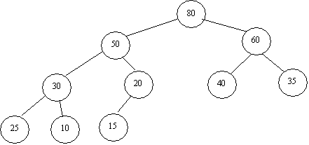
Figure 1.
Note that each parent node in the graph has a higher priority than either of its children, and that the priorities of sibling nodes are arbitrary in relation to each other. Given the structure shown above, we now must determine how to implement the Insert and Delete operations.
Insert into a Heap
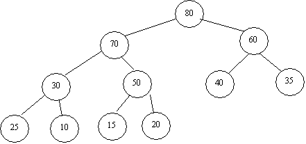
Insert into a heap is always done at the leftmost available leaf at the bottom level (in the example above, at the right child of node 20). However, after an insert is made into this position, the resulting graph may no longer be a heap, so the heap property needs to be reestablished. In this case we must push the new node "up" the head until it reaches its appropriate position. This is done through the following pseudocode:
upheap
{
while (priority(parent(v)) < priority(v))
swap(v, parent(v))
}
The idea is that eventually v will reach a point where its parent has a higher priority than it does, which has restored the heap property. Note that we don't even have to consider the priorities of sibling nodes, since the partial ordering of the heap only considers the parent-child relationship. As an example, if we were to insert 70 into the heap from Figure 1, we would get the resultant heap shown below:
Delete from a Heap
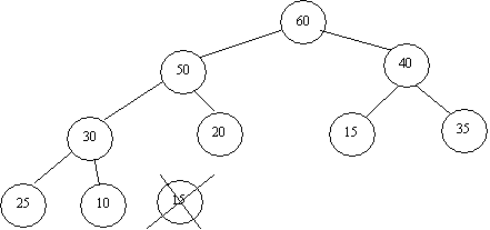
Delete from a heap is always the root node, since that is the node with the highest priority. However, as you are aware from binary search trees, deleting a node with two children in a binary tree is not a trivial task, since the structure of the subtrees would have to be altered to allow for all links to be made correctly. Instead, we will copy the last leaf value to the root node, and then (physically) delete the leaf node (which is a much simpler deletion procedure). Now the heap property must be reestablished, this time by moving the new root value down the tree until it reaches its proper spot. This can be accomplished by following the pseudocode below:
downheap
{
while (priority(v) < priority(either_child_of_v))
swap(v, higher_priority_child(v))
}
In this case, since we are moving the value down the tree, we must consider both children before swapping, since the resultant parent must have a higher priority than either of its children. As an example, if we were to do a Delete(Max) from the heap of Figure 1, the resultant heap would be:
Implementing a Heap
Although heaps are special binary trees, since they are complete trees it is more efficient to store and access them using arrays rather than using pointers and nodes. Complete binary trees have the nice property that if the nodes are numbered level by level starting at the root, the numbers of a parent node and its children nodes will be related in the following ways:
Consider node i in the tree
Parent(i) = i/2 // assuming integer division
Left_Child(i) = 2i
Right_Child(i) = 2i + 1
Consider again the heap in Figure 1, now numbered level-by-level as shown below:
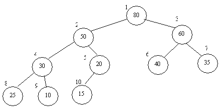
You can verify that the parent/child index relations hold as specified above. These relationships allow us to store the tree within an array as shown below:
|
Index |
1 |
2 |
3 |
4 |
5 |
6 |
7 |
8 |
9 |
10 |
11 |
|
Value |
80 |
50 |
60 |
30 |
20 |
40 |
35 |
25 |
10 |
15 |
|
In the array above, index 11 is left open and would be the location of the next Insert value prior to the call to upheap. Naturally, the array would have to be oversized or dynamically resized to handle a heap whose number of nodes varies greatly, but still it is faster and generally more memory-efficient than using dynamic nodes (no extra pointer links required).
Run-time
The run-time of Insert and Delete in the heap described above is clearly proportional to the height of the tree (think about what upheap and downheap must do). Since the tree is a complete binary tree, we know that for n nodes its height is proportional to lg n. Thus, both Insert and Delete using a heap require Theta(lg n) time. For a sequence of n operations, this gives us a total run-time of Theta(n lg n), which is a good improvement over the Theta(n2) time required by either the sorted array or unsorted array implementation.
Adding Change to the mix
In the PFS MST and shortest path algorithms, an item in the priority queue can be updated with a new priority (possibly multiple times). This can be done in three steps:
1) Find the item to be updated
2) Change the value (if necessary)
3) Reestablish the heap property
The heap implementation shown above (and indeed, any traditional priority queue implementation) does not efficiently support the Find operation. Since the data is only partially ordered, to find a specific item we must do an exhaustive search, requiring Theta(n) time. However, this deficiency can be overcome through the use of indirection, as discussed in Chapter 11 of the text and in the pq.h handout. The basic idea is that we keep an array indexed on the vertex index values that is storing the position of those vertices within the heap. Through this extra array we can Find a vertex within the heap in Theta(1) time. Then we simply change the priority (if necessary) and call upheap or downheap depending upon whether we increased or decreased the priority (for the PFS algorithm, we would only increase the priority).