c10dow - page 1 of 1

Chapter 10 Tables

C. R. Dow, Feng Chia University, Taiwan (crdow@fcu.edu.tw)

Chapter Content:

10.1 Introduction

10.2 Rectangular Arrays

10.3 Tables of Various Shapes

10.3.1 Triangular Tables

10.3.2 Jagged Tables

10.3.3 Inverted Tables

10.4 The Symbol Table Abstract Data Type

10.5 Static Hashing

10.5.1 Hashing Function

10.5.2 Collision Resolution with Open Addressing

10.5.3 Collision Resolution by Chaining

10.6 Dynamic Hashing

10.6.1 Dynamic Hashing Using Directories

10.6.2 Directoryless Dynamic Hashing

10.7 Conclusions

Exercises

10.1 Introduction

In Chapter 4, we showed the problem of searching a list to find a specific entry and

discussed two well-known searching algorithms: sequential search and binary search.

By using key comparisons alone, we can complete a binary search of n items in fewer

than log(n) comparisons. In this chapter, we begin with normal rectangular arrays, and

then extend to the study of hash tables which can break the log(n) barrier of binary

search. The average time complexity of hashing is bounded by a constant that does

not depend on the size of the table.

10.2 Rectangular Arrays

Nearly all high-level languages provide convenient schemes to access rectangular

arrays, so the programmer generally does not need to worry about the implementation

details of rectangular arrays. Computer storage is practically arranged in a contiguous

sequence, so for every access to a rectangular array, the computer converts the

location to a position along a line. In this section, we will talk about the details of the

ordering process (see Fig. 10.1).

Fig. 10.1 Contiguous sequence

Row-Major and Column-Major Ordering

The normal way

to read a rectangular array is from left to right of each row or from

top to bottom of each column. We can read the entries of the first row from left to

right, then read the entries of the second row, and so on until the last row has been

read. Most systems store a rectangular array with the order, called row-major

ordering (see Fig. 10.2). Similarly, if a rectangular array is read from top to bottom of

each column, this method is called column-major ordering (see Fig. 10.2).

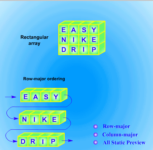
Fig. 10.2 Row- and column-major ordering

Indexing Rectangular Arrays

In general, an index (i, j) is translated into a memory address where the corresponding

entry of the array will be stored. A formula for the calculation can be derived as

follows. Suppose we use row-major ordering and the rows are numbered from 0 to

m-1 and the columns from 0 to n-1. Thus, the array will have mn positions, and the

range is from 0 to mn-1. With this information, we can define a formula to convert an

index to a position. On the first row, (0, 0) goes to position 0, (0, j) goes to position j,

and (0, n-1) goes to position n-1 as shown in Fig. 10.3(a)

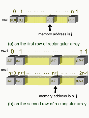
Fig. 10.3 Indexing Rectangular Arrays

On the second row, the first entry of the second row, (1, 0), comes after (0, n-1), and it

goes into position n (see Fig. 10.3(b)). Also, we can see that (1, j) goes to position n+j

and (2, j) goes to position 2n+j, so the formula is

Entry (i, j) goes to position ni + j.

The above formula, which gives the sequential location of an array entry, is called an

index function. According to this function, we can calculate the memory position

accurately.

Variation: An Access Table

Although calculating the index function of a rectangular array is simple, it might be

not very efficient on some small machines to do multiplication.

Thus, we can use the

following method to eliminate the multiplications.

Assume the size of a rectangular array is m*n. This method is to keep an auxiliary

array, a part of the multiplication table for n. The array will contain the values

0, n, 2n, 3n, …, (m-1)n

We can use the small array to keep a reference to each column of the rectangular array.

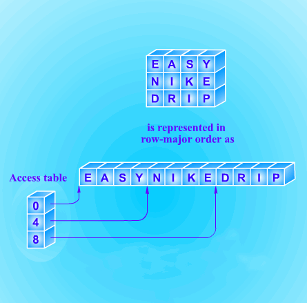
It will be calculated only once, and it can also be calculated by addition on the small

machine. The array is normally much smaller than the rectangular array, so that it can

be placed in memory permanently without wasting too much space.

Fig. 10.4 Access table for a rectangular array

This auxiliary table provides an example of an access table (see Fig. 10.4). In general,

an access table, also called access vector, is an auxiliary array used to find data stored

somewhere else.

10.3 Tables of Various Shapes

We may not store data into every position of a rectangle array. If we define a matrix to

be an array of numbers, then some of the positions will be 0 or no data, such as

tri-diagonal matrix, lower triangular matrix, etc. Several matrix examples are shown

in Fig. 10.5. In this section, we study schemes to implement tables of various shapes

to eliminate unused space in a rectangular array.

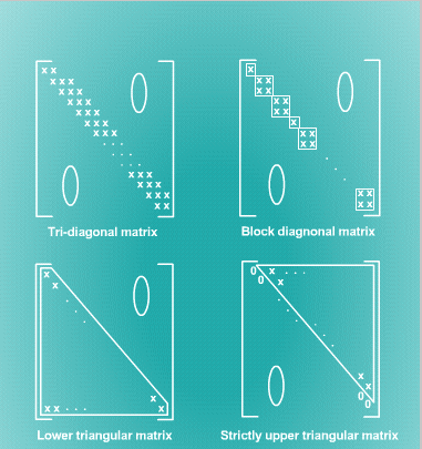
Fig. 10.5 Matrices of various shapes

10.3.1 Triangular Tables

As shown in Fig. 10.6, all indices (i,j) of the lower triangular table are required to

satisfy i >= j. A triangular table can be implemented in a contiguous array by sliding

each row out after the one above it (please press the “play it” button in Fig. 10.6). To

create the index function, we assume the rows and the columns are numbered starting

with 0. We know the end of each row will be the start of the next row. Clearly, there is

no entry before row 0, and only one entry of row 0 precedes row 1. For row 2 there

are 1 + 2 = 3 preceding entries (one entry of row 0 and two entries of row 1), and for

row i there are

)

...

entries. Thus, the entry (i,j) of the triangle matrix is

)

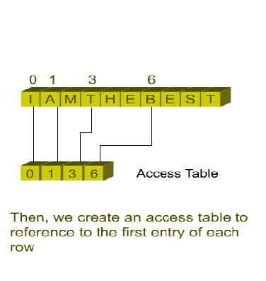
Fig. 10.6 Contiguous implementation of a triangular table

As we did for rectangular arrays in Section 10.2, we can avert multiplications and

divisions by setting up an access table. Each entry of the access table makes a

reference to the start position of each row in the triangular table. The access table will

be calculated only once at the begging of the program, and it will be used again and

again. Notice that even the initial calculation of the access table requires only addition

but not multiplication or division to calculate its entries in the following order.

0, 1, 1+2, (1+2)+3, …

10.3.2 Jagged Tables

In an ordinary rectangular array, we can find a simple formula to calculate the

position, because the length of each row is the same. For the case of jagged tables, the

relation between the position of a row and its length is unpredictable.

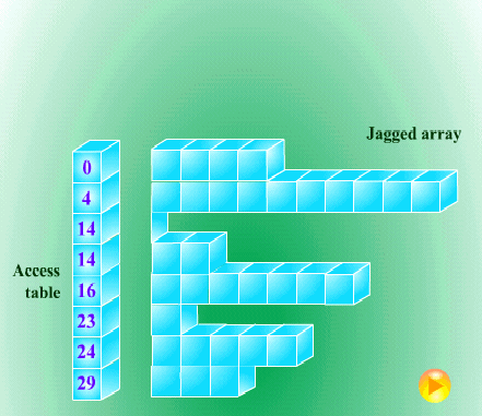
Fig. 10.7 Access table for jagged table

Since the length of each row is not predictable, we cannot find an index function to

describe it. However, we can make an access table to reference elements of the jagged

table. To establish the access table, we must construct the jagged table in a natural

order, starting from 0 and beginning with its first row. After each row has been

constructed, the index of the first unused position of the continuous storage is entered

as the next entry in the access table. Figure 10.7 shows an example of using the access

table for jagged table.

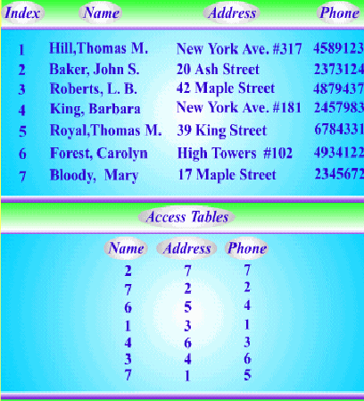
10.3.3 Inverted Tables

Multiple access tables can be referred to a single table of records by several different

keys forthwith. In some situations, we may need to display different information

sorted by different keys. For example, if a telephone company wants to publish a

telephone book, the records must be sorted alphabetically by the name of the

subscriber.

But to process long-distance charges, the accounts must be sorted by

telephone number. To do routine maintenance, the company also needs to sort its

subscribers by address, so that a repairman may work on several lines with one trip.

Therefore, the telephone company may need three copies of its records, one sorted by

name, one sorted by number, and one sorted by address. Notice that keeping three

same data records would be wasteful of storage space. And if we want to update data,

we must update all the copies of records and this may cause erroneous and

unpredictable information to the user.

The multiple sets of records can be avoided by using an access table.

We can even

find the records by any of the three keys. Before the access table is created, the index

of records is required. According the index number, we can replace data with the

index number in the access table. Thus, the table size can be reduced and it will not

waste too much storage space. Figure 10.8 shows an example of multikey access table

for an inverted table.

Fig. 10.8 Multikey access tables: an inverted table

10.4 The Symbol Table Abstract Data Type

Previously, we studied several index functions used to locate entries in tables, and

then we converted them to access tables, which were arrays used for the same purpose

as index functions. The analogy between functions and table lookup is very close. If

we use a function, an argument needs to be given to calculate a corresponding value;

if we use a table, we start with an index and look up a corresponding value from the

table.

Functions and Tables

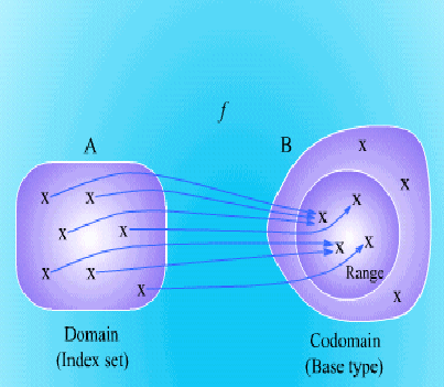
Let us start from the definition of a function (see Fig. 10.9). In mathematics, a

function is defined in terms of two sets and an accordance from elements of the first

set to elements of the second set. If f is a function from set A to set B, then f assigns to

each element of A unique element of B. The set A is called the domain of f, and the

set B is called the codomain of f.

Table access begins with an index and uses the table to look up a corresponding value.

Thus, we call the domain of a table the index set, and the codomain of a table the base

type or value type. For instance, we may have the array declaration:

int array[n];

Then the index set is the set of integers between 0 and n-1, and the base type is the set

of integers.

Fig. 10.9 The domain, codomain, and range of a function

An Abstract Data Type

Before we define table as a new abstract data type, let us summarize what we know. If

we have a table with index set I and base type T, the table is a function from I into T

and with the following operations.

(1) Table access: Given an index argument in I, we can reply a corresponding value in

(2) Table assignment: Modify the value at a specified index in I to a new value.

These two operations can be easily

implemented by the C language or some other

languages. Comparing with another abstract data type, list, an element can be inserted

into the list or removed from it. There is no reason why we cannot allow the

possibility of further operations. Thus, various operations for table are defined as

follows.

(3) Creation: Set up a new function.

(4) Insertion: Add a new element x to the index set I and define a corresponding value

of the function at x.

(5) Deletion: Delete an element x from the index set I and confine the function to the

resulting smaller domain.

(6) Clearing: Remove all elements from the index set I, so there is no remaining

domain.

The fifth operation might be hard to implement in C, because we cannot directly

remove any element from an array. However, we may find some ways to overcome it.

Anyway, we should always be careful to write a program and never allow our

thinking to be limited by the restrictions of a particular language.

Comparisons

The abstract data types of list and table can be compared as follows. In the view of

mathematics, the construction for a list is the sequence, and for a table it is the set and

the function. Sequences have an implicit order: a first element, a second, and so on.

However, sets and functions have no order and they can be accessed with any element

of a table by index. Thus, information retrieval from a list naturally invokes a search.

The time required to search a list generally depends on how many elements the list

has, but the time for accessing a table does not depend on the number of elements in

the table. For this reason, table access is significantly faster than list searching in

many applications.

Finally, we should clarify the difference between table and array. In general, we shall

use table as we have defined it previously and restrict the term “array” to mean the

programming feature available in most high-level languages and used for

implementing both tables and contiguous lists.

10.5 Static Hashing

10.5.1 Hashing Function

When we use a hash function for inserting the data (a key, value pair) into the hash

table, there are three rules must be considered. First of all, the hash function should be

easy and quick to compute, otherwise it will waste too much time to put data into the

table. Second, the hash function should achieve an even distribution of all data (keys),

i.e. all data should be evenly distributed across the table. Third, if the hash function is

evaluated more times of the same data, the same result should be returned. Thus, the

data (value) can be retrieved (by key) without failure.

Therefore, a selection of hash function is very important. If we know the types of the

data, we can select a hash function that will be more efficient. Unfortunately, we

usually don’t know the types of the data, so we can use three normal methods to set

up a hash function.

Truncation

It means to take only part of the key as the index. For example, if the keys are more

than two digit integers and the hash table has 100 entries (the index is 0~99), the hash

function can use the last two digits of the key as the index. For instance, the data with

the key, 12345 will be put into the 45th entry of the table.

Folding

It means to partition the key into many parts and then evaluate the sum of the parts.

For the above example, the key 12345 can be divided into three parts: 1, 23, and 45.

The sum of the three parts is 1 + 23 + 45 = 69, so we can put the data into the 69th

entry of the table. However, if the sum is larger than the number of entries, the hash

function can use the last two digits as the index, just like the truncation hash function

described above.

Modular Arithmetic

It means to divide the key by the size of the index entries, and take the remainder as

the result. For the above example, the key 12345 can be divided by the number of

entries 100, i.e. 12345 / 100 = 123 … 45, the remainder 45 will be treated as the index

of the table.

Sometimes, the key is not an integer number, therefore the hash function must convert

the key to an integer. In the C example of Fig. 10.10, the key is a string, so we can add

the values of the characters (a string is a set of characters) as the key.

Fig. 10.10 hashing by using a character string

10.5.2 Collision Resolution with Open Addressing

In the previous section, we have described the hash function. In some situations,

different keys may be mapped to the same index. Therefore, we will describe in this

section a number of methods to resolve this collision.

Linear Probing

The simplest method to resolve the collision is to search the first empty entry of the

int string2integer(char *key)

{

int ikey = 0;

while (*key)

ikey += *(key++);

return ikey;

}

/* function: hash, using an integer as key */

int hash (int key)

{

// some hash function implementation

return key & TABLE_ENTRIES_NUMBER;

// modular arithmetic implementation

}

/* function: hash, using a string as key */

int stringHash (char *key)

{

int ikey = string2integer(key);

return hash(ikey);

}

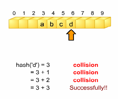
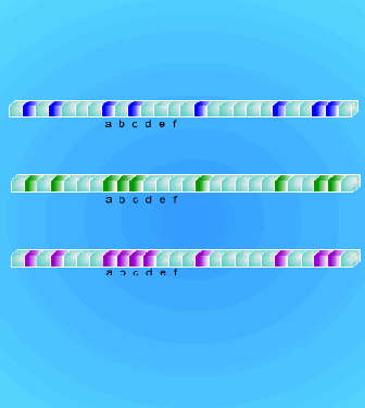
table. Of course, the starting entry of search depends on the index returned by the

hash function. When the starting entry is not empty, this method will sequentially

search the next entry until it reaches an empty entry. If the entry is the end of the table,

its next entry is the first entry of the table. An example of this scheme is shown in Fig.

10.11.

Fig. 10.11 Linear probing

Clustering

Fig. 10.12 Clustering

The problem of linear probing happens when the table becomes about half full, there

is a tread toward clustering; that is, there are many long strings of non-empty entries

in the table. Consider the example in Fig. 10.12, the color position means a filled

entry. In the first situation, if we insert a data with a key ‘a’ (denoted as DATA(a)), the

linear probing will search 2 times (the ‘b’ entry is empty). In the next situation, we

insert DATA(a) again, this method will waste 4 times. The last situation, it will search

5 times. If we discuss the average times of inserting DATA(a), DATA(b), DATA(c)

and DATA(d) in these three situations:

Situation 1:

( 2 + 1 + 2 + 1 ) / 4 = 1.5 times

DATA(a) DATA(b) DATA(c) DATA(d)

Situation 2:

( 4 + 3 + 2 + 1 ) / 4 = 2.5 times

DATA(a) DATA(b) DATA(c) DATA(d)

Situation 1:

( 5 + 4 + 3 + 2 ) / 4 = 3.5 times

DATA(a) DATA(b) DATA(c) DATA(d)

Just like the name, linear probing, the average overhead of searching an empty entry

is also linear, i.e. O(n) for the clustering situation.

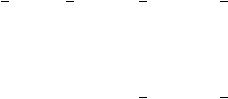
Rehashing and Increment Functions

In order to resolve the problem of linear probing, we can provide more than one hash

function. When a collision occurs, another hash function could be used (see Fig.

10.13). This method is called rehashing and an increment functions is derived from

this method. We treat the second hash function as an increment function instead of a

hash function, that is, when a collision occurs, the other increment function is

evaluated and the result is determined as the distance to move from the first hash

position (see Fig. 10.14). Thus, we wish to design an increment function that depends

on the key and can avoid clustering.

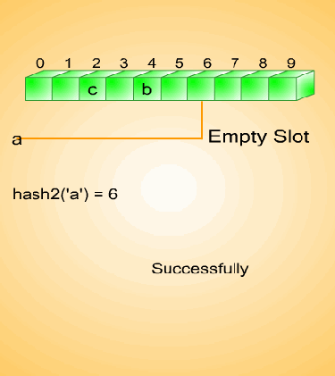
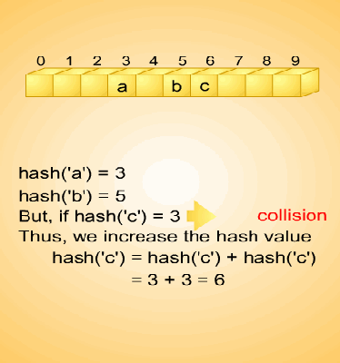
Fig. 10.13 Rehashing

Fig. 10.14 Increment function

Key-Dependent Increments

As just mentioned, we can design an increment function that depends on the key. For

instance, the key can be truncated to a single character and use its code as the

increment. In C, we might write

increment = *key; //or increment = key[0];

Quadratic Probing

If the hash function is h and increment function is i², the method probes the table at

locations h + 1, h + 4, h+9, i.e. at location h + i²(%HASHSIZE) when there is a

collision. In Fig. 10.14, we can use the f(i)= i² as the increment function.

Furthermore, how to select an appropriate HASHSIZE is very important. In general,

we use a prime number for HASHSIZE to achieve better performance.

Random Probing

This method uses a random number as the increment. Of course, the random number

must be the same every time when we retrieve the same value (namely by the same

key) from the table or put the same value into the table. This is a very simple thing to

reach the goal, if we use the same seed and the same sequence value, the random

number will be the same. The seed and sequence values can be obtained based on the

portion of the key values.

10.5.3 Collision Resolution By Chaining

Up to this section we only use the contiguous storage to store the data (the key and

value), but the fixed-size storage is not good when the number of data records keep

changing. On the contrary, it is more appropriate for random access and refers to

random positions. An example is illustrated in Fig. 10.15 and in the following we will

describe the advantages and disadvantages of the chaining scheme.

Fig. 10.15 Collision resolution by chaining

Advantages of Chaining

Space Saving and Overflow

The first advantage of chaining is space saving. If we use a contiguous storage, we

need to maintain a large size of storage to avoid overflow. That is, if we put data into

a table and there is no space, we may need to renew a larger array and re-insert the

data (old data in table and new data not inserted yet). It is inefficient because of

reconstructing (renew) and copying (re-insert) operations. On the contrary, the

chaining skill will use a pointer to refer to the next data that has the same key

(collision occurred), so the origin storage does not need a large space to avoid

overflow.

Collision Resolution

The second advantage is that when the collision occurs, we do not use any function to

deal with. We only use a pointer to refer the new data and use a single hash address as

a linked list to chain the collision data. Clustering is no problem at all, because keys

with distinct hash addresses always go to distinct lists. Figure 10.15 illustrates this

situation.

Deletion

Finally, deletion becomes s quick and easy means for a chained hash table. The

deletion operation does the same way as deletion from a linked list.

Disadvantages of Chaining

Because the chaining structure has to remain a reference as a pointer to refer the next

data that contains the same key, the structure is larger than the entry of static table

(used in previous sections). Another problem is that when the chain is too long, to

retrieve the final entry of this chain is too slow.

10.6 Dynamic Hashing

Motivation for Dynamic Hashing

The skill mentioned in last section is not efficient for the situation where the number

of data records is substantially changed following by the time, e.g. DBMS. Because

the skill uses a static array to maintain the table, the array may need to store the data

or take the entry as a linked list header (chaining). Regardless of which situation, if

the array is too large, the space could be wasted; but if the array is too small, an

overflow will occur

frequently (open address). If the chain is too long, it will

reconstruct a new hash table and rehash the table so it is very inefficient. That is, the

goal of dynamic hashing (or say extendible hashing) is to remain the fast random

access of the traditional hash function and extend the function and make it not

difficult to dynamically and efficiently adjust the space of hash table.

10.6.1 Dynamic Hashing Using Directories

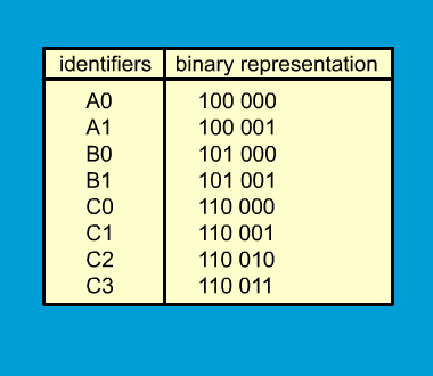
Fig. 10.16 The presentation of every letter

In this section, we will use an example to describe the principle. We assume the key

of data is two letters and each letter is represented by three bits. An example is shown

in Fig. 10.16. At the beginning of initiation, we put the data (the key) into a four entry

table, every entry can save two keys. We use the last two bits as the key and determine

which entry the data should be saved in. Then, we put the keys A0, B0, C2, A1, B1

and C3 into the table. Based on the last two bits of the key, A0 and B0 are put into the

same entry, A1 and B1 are put into the same entry, and C2 and C3 are put into the

distinct entry separately.

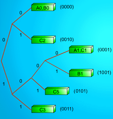
Fig. 10.17 An insertion example

Now, we insert a new data C5 into the table. Since the last two bits of C5 is equal to

the last two bits of A1 and B1 and every entry can only save two keys, we will branch

the entry into two entries and use the last three bits to determine which one should be

saved in which entry. As shown in Fig. 10.17, if we insert a new data again, it will

perform the same procedure as before.

In this example, two issues are observed. First, the time of access entry is dependent

on the bits of the key. Second, if the partition of the key word is leaned, the partition

of the table is also leaned.

In order to avoid waiting too long to search the long list, each entry can be mapped to

a directory, as shown in Fig. 10.18. Each subfigure of Fig.10.18 corresponds to each

subfigure of Fig. 10.17. Notice that the directory is a pointer table. If we need k bits to

substitute the key, the directories will have 2

entries.

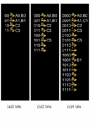
Fig. 10.18 Directory

In Fig. 10.18(a), because we only use two bits to represent four keys, the directories

also need only four entries. When inserting C5, C5’s last two bits equals A1 and B1

(01), but the entry (01) has two pointers (pointing to A1 and B1). Thus, the directory

must be extended as shown in Fig. 10.18(b), where C5 would be put into entry 101.

Finally, we put C1 into table, the last three bit is 001 and equals to A1 and B1, and the

entry 001 has two pointers to indicate A1 and B1’s pointers, so we need to extend this

table again, as shown in Fig. 10.18(c). Although the last three bits are the same (001),

the last four bits of A1 and C1 are the same (0001). However, B1 is (1001), so B1 will

be put into the 1001th entry.

Using this approach, the directory will be dynamically extended or shrank.

Unfortunately, if these keys do not distribute uniformly, the directory will become

very large and most of the entries are empty, as shown in Fig. 10.18(c). To avoid this

situation, we may convert the bits into a random order and it can be performed by

some hash functions.

10.6.2 Directoryless Dynamic Hashing

In the previous section, we need a directory to put the pointers of the data. In this

section, we assume that there is a large memory that is big enough to store all records,

then we can eliminate the directory.

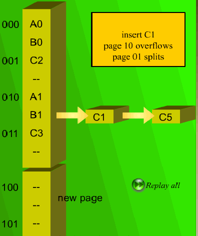
When an overflow occurs, we need to increase the memory space, but this will waste

too much memory. To avoid the overflow, we only add one page and rehash the table.

As shown in Fig. 10.19, when we insert a new data C5 the table will be extended.

Despite rehashing, the new page is empty. Once again, if we insert a value C1 again,

the same situation occurs and the new page is still empty. So this approach can avoid

creating many new pages (two times to the original one). Sometimes, the new page is

still empty, i.e., the new page is not effective.

Fig. 10.19 A directoryless hashing example

The general method to deal with overflow problem is one of the traditional rehash

functions, just like the open addressing.

10.7 Conclusions

In this chapter, we describe the table of various shapes, including triangular tables,

jagged tables and inverted tables, in the former sections. And we also describe the

technique to implement the abstract data type of the table. In the later sections, we

focus on the data retrieval from the table. So we explain many hashing functions, such

as static hashing (truncation, folding, modular, etc.) and dynamic hashing (using

directories and directoryless), and approaches of collision resolution, such as open

addressing (linear probing, quadratic probing, etc.) and chaining.

Exercises

Beginner’s Exercises

Multiple-choice questions:

1. Suppose there is an integer array M (5,8), the address of M (0,0), M (0,3) and M

(1,2) are 100,106 and 120, respectively. What is the address of M (4,5)? (a) 174 (b)

164 (c) 168 (d) 186 (e) None of above.

Assume each integer takes one memory location to store. Consider the array

declaration: var A : array[1..5, 20..25 ,10..15] of integer; Assume the array is stored

in row major order. If A[4,25,15] is stored in location 1999, what is the location of

Assume that A is an n*n matrix with A(i,j)=0, for i+j ? n+2. What are the

maximum number nonzero elements in A? (a)n*(n+1)/2 (b) n*(n-1)/2 (c)n² (d) n²/2

(e)None of above.

4. Which is not a method of setting up a hash function?

(a)Truncation (b)Modular Arithmetic (c)Chaining (d)Folding (e)None of above.

5. Consider the symbol table of an assembler, which data structure will make the

searching faster (assume the number of symbols is greater than 50 ).

(a)sorted array (b)hashing table (c)binary search tree (d)unsorted array (e)linked

list.

6. A hash table contains 1000 slots, indexed from 1 to 1000. The elements stored in

the table have keys that range in value from 1 to 99999. Which, if any, of the

following hash functions would work correctly?

(a)key MOD 1000 (b)(key-1) MOD 1000 (c)(key+1) MOD 999 (d)(key MOD

1000)+1 (e)None of above.

7. Which is not the method of resolving collision when handling hashing operations?

(a)Linear probing (b)Quadratic probing (c)Random probing (d)Rehashing (e)None

of above.

8. Consider the following 4-digit employee numbers: 9614, 1825 Find the 2-digit hash

address of each number using the midsquare method. The address are (a)14,06

(b)30,06 (c)28,15 (d)28,30 (e)None of above.

9. Continue from 8. Find the 2-digit hash address of each number using the folding

method without reversing (shift folding). The address are (a) 61,82 (b)10,43

10. Which is not the application of using hashing function?

(a)Data searching (b)Data store (c)Security (d)Data compression (e)None of above.

Yes-no questions:

1. If a rectangular array is read from top to bottom of each column, this method is

called row-major ordering.

2. We can use triangular tables, jagged tables and inverted tables to eliminate unused

space in a rectangular array.

3. If f is a function from set A to set B, then f assigns to each element of A a unique

element of B. The set A is called the codomain of f, and the set B is called the

domain of f.

4.The time required to search a list generally does not depend on how many elements

the list has, but the time for accessing a table depends on the number of elements in

the table. For this reason, table access is significantly slower than list searching in

many applications.

5. A selection of hash function is very important. If we know the types of the data, we

can select a hash function that will be more efficient. Furthermore, we always know

the types of the data, so we can set up a hash function easily.

6. We can provide more than one hash function to resolve the clustering problem of

linear probing. When a collision occurs, another hash function could be used. This

method is called rehashing and an increment functions is derived from this method.

7. The chaining skill uses a pointer to refer to the next data, which has the same key

(collision occurred), so the origin storage does not need a large space to avoid

overflow. When the chain is long, it is easy to retrieve the final entry of this chain.

8. The goal of dynamic hashing (or say extendible hashing) is to remain the fast

random access of the traditional hash function and extend the function and make it

not difficult to dynamically and efficiently adjust the space of hash table.

9. In the method of dynamic hashing using directories, the directory is a pointer table.

If we need n bits to substitute the key, the directories will have 2

n+1

entries.

10. We can find out that the space utilization for directoryless dynamic hashing is not

good. Because some extra pages are empty and yet overflow pages are being used.

Intermediate Exercises:

11. Write a program that will create and print out a lower triangular table. The input is

a number N (e.g.4) and the table will look like the following.

1 0 0 0

2 3 0 0

4 5 6 0

7 8 9 10

12. Please design a hash function that can be used to save a character into a hash table

(array) and this hash function should be used to do the searching. (Please use the

linear probing technique to solve the collision problem.)

13. Please design a hash function that can be used to save an integer into a hash table

(array) and this hash function should be used to do the searching. (Please use the

chaining technique to solve the collision problem.)

Advanced Exercises:

14. A lower triangular matrix is a square array in which all entries above the main

diagonal are 0. Describe the modifications necessary to use the access table method to

store an lower triangular matrix.

15. In extendible hashing, given a directory of size d, suppose two pointers point to

the same page. How many low-order bits do all identifiers share in common? If four

pointers point to the same page, how many bits do the identifiers have in common?

16. Prove that in directory-based dynamic hashing a page can be pointed at by a

number of pointers that is a power of 2.

17. Devise a simple, easy-to-calculate hash function for mapping three-letter words to

integers between 0 and n-1, inclusive. Find the values of your function on the words

POP LOP RET ACK RER EET SET JET BAT BAD BED

for n = 11, 15, 19. Try for as few collisions as possible.

18. Based on Exercise 17, write a program that can insert these words (PAL, LAP, etc.)

into a table, using the tree structure and arrays as show in Fig. 10.17 and 10.18,

respectively.