CS1674: Homework 6 - Programming

1. [10 pts] Given an RGB image, perform clustering in the 3-dimensional RGB space, and map each pixel in the input image to its nearest k-means center. That is, replace the RGB value at each pixel with its nearest cluster's average RGB value. For example, if you set k=2, you might get:
   
   Since these average RGB values may not be integers, you should round them to the nearest integer (1 through 255). Use the following form:
   function [outputImg, meanColors, clusterIds] = quantizeRGB(origImg, k)
   where origImg and outputImg are RGB images of type uint8, k specifies the number of colors to quantize to, and meanColors is a kx3 array of the k centers (one value for each cluster and each color channel). clusterIds is a numpixelsx1 matrix (with numpixels = numrows * numcolumns) that says which cluster each pixel belongs to. Matlab tip: if the variable im is a 3d matrix containing a color image with numpixels pixels in each color channel, X = reshape(im, numpixels, 3); will yield a matrix with the RGB features as its rows.


2. [2 pts] Write a function to compute the Euclidean distance between the original RGB pixel values and the quantized values (this is also called sum-of-squared-differences or SSD error). Use the following form:
   function [error] = computeQuantizationError(origImg, quantizedImg)
   where origImg and quantizedImg are both RGB images of type uint8, and error is a scalar giving the total SSD error across the image.


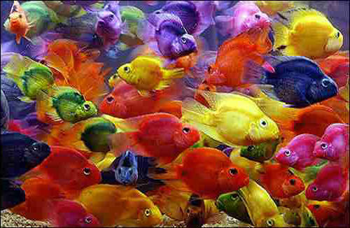
3. [8 pts] Write a script colorQuantizeMain.m that calls all the above functions appropriately using the provided image fish.jpg, and displays the results. Illustrate the quantization with at least three different values of k. Label all plots clearly with titles. In a text file explanation.txt, briefly answer the following: How and why does the SSD differ based on the value of k?

1. [10 pts] function [edges] = detectEdges(im, threshold) -- A function to compute edges in an image. im is the input image in uint8 type and in color, and threshold is a user-set threshold for detecting edges. edges is an Nx4 matrix containing 4 numbers for each of N detected edge points: N(i, 1) is the x location of the point, N(i, 2) is the y location of the point, N(i, 3) is the gradient magnitude at the point, and N(i, 4) is the gradient orientation (non-quantized) at the point.
   Instructions:
   • In this function, simply compute the gradient magnitude and orientation at each pixel, and only return those (x, y) locations with magnitude that is higher than the threshold. Use the magnitude and orientation equations (and reuse as much code as possible) from HW4P (but see an exception below).
   • At the end, display, save, and include in your writeup the thresholded edge image for an image of your choice, as in slide 19 here (but for simplicity, show edges with intensity equal to their magnitude, and non-edges as black i.e. intensity 0).
   Tips:
   • Remember that the x direction corresponds to columns and the y direction corresponds to rows.
   • For the sake of the next part, try using atan instead of atand -- I had better success with that.
   • Useful functions: find, ind2sub.


2. [15 pts] function [centers] = detectCircles(im, edges, radius, top_k) -- A function to find and visualize circles from an edge map. im, edges are defined as above, radius specifies the size of circle we are looking for, and top_k says how many of the top-scoring circle center possibilities to show. The output centers is an Nx2 matrix in which each row lists the x, y position of a detected circle's center.
   Instructions:
   • Follow the pseudocode on slide 38 here, and use the gradient orientation you computed in the function above.
   • Use this line at the end of your function to visualize circles: figure; imshow(im); viscircles(centers, radius * ones(size(centers, 1), 1));.
   Tips:
   • Consider using ceil(a / quantization_value) and ceil(b / quantization_value) (where, for example, quantization_value can be set to 5) to easily figure out quantization/bins in Hough space. Don't forget to multiply by quantization_value once you've figured out the Hough parameters with most votes, to find out the actual x, y location corresponding to the selected bin.
   • Ignore circles whose centers are outside the image.
   • Useful Matlab functions: sort, ind2sub, ceil, sin, cos, viscircles, impixelinfo.


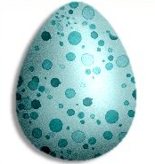
3. [5 pts] Demonstrate the function applied to the provided images jupiter.jpg and egg.jpg. Display the images with detected circle(s), labeling the figure with the radius, save your image outputs, and include them in your submission. You can use impixelinfo to estimate the radius of interest manually.